
Building Management System (BMS) Software: Every Module, Every Calculation, and How It All Connects
A researched, module-by-module breakdown of building management system software: the five-layer hierarchy, the maths each module runs, and how the modules connect. 2026 guide.
On this page
Almost every large building runs on software most people never see. It decides when the heating starts, how much fresh air each room gets, which chiller runs, when a fault becomes a work order, and what the tenant is charged for electricity. That software is called a building management system (BMS), and it is suddenly one of the most wanted categories in property technology.
This paper maps the whole thing. It is not a build guide. It is a reference for the parts: the hierarchy of modules, what each one does, the calculations it runs, and exactly how it connects to the others. If you own, operate, invest in, or plan to build software for buildings, this is the structure you need in your head.
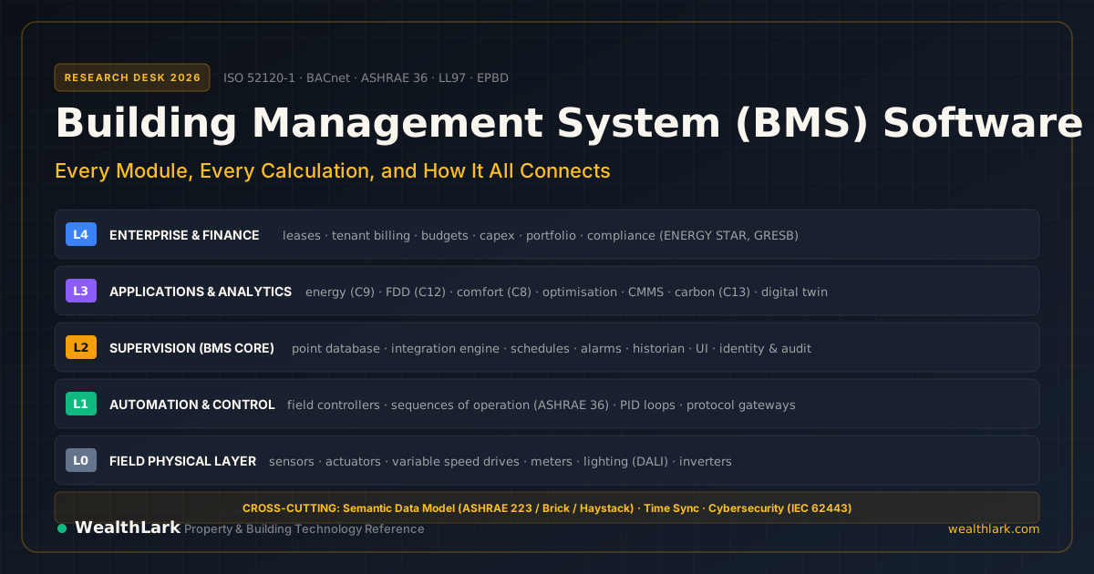
A modern BMS spans five discrete functional layers: L0 Field Devices, L1 Automation & Control, L2 Supervision (Core BMS), L3 Applications & Analytics, and L4 Enterprise & Finance. Real-time control loops run in seconds at L1 to guarantee physical fail-safe autonomy, while cloud analytics and capital planning execute at L3/L4. The financial lever is direct: operating savings flow straight into Net Operating Income (NOI), where every $1.00 of permanent operational reduction creates ~$16.67 in capitalized asset value at a 6.0% cap rate.
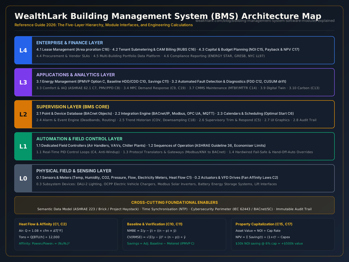
How to use this paper. Section 3 gives the five-layer map. Section 4 walks every module with what it does, what it calculates and what it talks to. Section 5 holds the formulas with worked examples. Section 6 shows how data actually moves between modules. Sections 7 and 8 cover standards, regulation and the money.
1. What a BMS is, and the words people confuse with it
Vendors and standards bodies use overlapping names. Here is how they differ in practice.
| Term | What it is | Typical scope |
|---|---|---|
| BMS | Software and hardware that monitor and control building systems from one place | HVAC, lighting, metering, access, alarms, reporting |
| BAS / BACS | The automation and control layer (EU law says “building automation and control system”) | Controllers, sensors, sequences that run the plant |
| EMS / EMIS | Energy management (information) system | Metering, baselines, savings, bills |
| CMMS | Computerised maintenance management system | Assets, work orders, preventive maintenance |
| IWMS / CAFM | Integrated workplace or facility management | Space, leases, projects, maintenance, move management |
| Property management software | Tenant and money side of a building | Leases, rent, charges, accounting |
| Digital twin | A live data model of the building, often with simulation | Analytics, what-if testing, visualisation |
In this paper, BMS software means the whole stack, from the sensor at the bottom to the finance report at the top. That is how buyers now think about it, and it is why the category keeps growing.
2. Why everybody wants it right now
Four forces are pushing in the same direction:
- Money and market size. Analyst estimates vary a lot because they define the market differently. One research house puts the global BMS market at about US$21.1 billion in 2026, growing to about US$39.5 billion by 2032 (11.04% a year). Another projects US$72.7 billion by 2035 (13.1% a year). Treat these figures as a range, not an absolute fact. The direction is consistent: strong double-digit annual growth.
- Regulation in Europe. The recast Energy Performance of Buildings Directive (EU) 2024/1275 requires building automation and control systems in non-residential buildings with heating or cooling above 290 kW by the end of 2024, falling to 70 kW by the end of 2029. From May 2026, larger non-residential buildings also need to monitor indoor environmental quality. Commentators read the directive as wanting documented proof that automation improves energy performance, not just a system that exists. The reference standard is ISO 52120-1 (which replaced EN 15232-1) and grades automation from Class A (best) to Class D (non-automated).
- Regulation in the US. New York City’s Local Law 97 charges $268 for every metric ton of CO₂e above a building’s annual cap. Limits tighten sharply in 2030, and one tracker found that 43% of covered buildings already meet the 2030 limits on 2024 energy use. Analysts expect more than 40 US cities to have mandatory building performance standards by the end of 2026. Penalties are an operating cost that software can measure and reduce.
- Technology. Cloud platforms, cheap IoT sensors, AI-driven fault detection, model predictive control (MPC), and digital twins now make it practical to do things that used to need an expert on site. The main bottleneck is data, not algorithms. The US National Institute of Standards and Technology (NIST) describes mapping building data points to analytics tools as a labour-intensive process, which is why semantic standards (Section 7) matter so much.
3. The five-layer reference architecture
Every serious BMS can be described as five layers plus a few cross-cutting concerns. Data flows up as measurements. Commands flow down as setpoints, schedules and overrides.

L4  ENTERPRISE & FINANCE      leases · tenant billing · budgets · capex · portfolio · compliance reports
L3  APPLICATIONS & ANALYTICS  energy · fault detection · comfort & air quality · optimisation
                              maintenance · space · carbon · digital twin · security & fire interfaces
L2  SUPERVISION (BMS core)    point database · integration · schedules · alarms · historian · UI · users
L1  AUTOMATION                controllers · control loops · sequences of operation · gateways
L0  FIELD                     sensors · actuators · meters · drives · fixtures · chargers · inverters

    CROSS-CUTTING             semantic data model · identity & audit · time sync · cybersecurity · commissioning records
Three design rules explain almost every architecture decision in the stack:
- Fast loops live low. Control that must react in seconds runs in L1 controllers, so a network or cloud outage never stops the building running.
- Slow decisions live high. Optimisation, analytics and billing run on minutes, days or months and can sit safely in the cloud.
- Everything shares one vocabulary. If L3 cannot tell that “AHU-3 SAT” is a supply air temperature sensor, no analytics module will work without hand configuration.
| Layer | Typical time scale | Owner of the data | Fails safe by |
|---|---|---|---|
| L0 Field | milliseconds to seconds | Device | Spring-return valves and dampers, hardware limits |
| L1 Automation | 1 to 10 second control loops | Controller | Local sequences keep running without the network |
| L2 Supervision | seconds to 15 minutes | Point database | Controllers ignore a dead supervisor |
| L3 Applications | minutes to days | Analytics store | Application outage affects insight, not physical comfort |
| L4 Enterprise | days to months | Finance & lease systems | Manual accounting workflow continues uninterrupted |
Enterprise Building Automation, Energy Meters & Cloud Supervisory Solutions
4. The module catalogue, layer by layer
Each entry details what the module does, what it calculates (formula citations point to Section 5), and what it connects to.
Layer 0: Field devices
- 0.1 Sensors and meters. Temperature, humidity, CO₂, pressure, flow, current, occupancy, and revenue-grade energy meters turn physical phenomena into data.
- Calculates: Signal scaling (e.g. 4–20 mA or 0–10 V to engineering units like °C, psi, cfm), calibration offsets, and sensible/latent heat flow (C1).
- Connects to: Feeds L1 controllers directly via analog/digital inputs, or communicates to L2 over Modbus RTU/TCP, M-Bus, or pulse accumulators for submetering.
- 0.2 Actuators and drives. Modulating valves, damper actuators, and variable frequency drives (VFDs) physically move air, water, and power.
- Calculates: Position feedback tracking, drive frequency scaling to power consumption via affinity laws (C2).
- Connects to: Commanded directly by L1 controllers. Spring-return actuators enforce a physical safe state when control signal or main line power drops.
- 0.3 Subsystem devices. DALI-2 lighting fixtures, OCPP electric vehicle chargers, Modbus solar inverters, battery storage (BESS), and elevator/escalator banks.
- Connects to: Subsystems interface through protocol gateways or specialized vendor controllers, bridging native vendor protocols into BACnet or REST APIs.
Layer 1: Automation
- 1.1 Field controllers. Dedicated microcontrollers for air handlers (AHUs), variable air volume (VAV) terminal boxes, fan coil units (FCUs), and chiller/boiler central plants.
- Calculates: Real-time PID feedback loops (C4), airflow tracking, static pressure control, and safety freeze-stat interlocks.
- Connects to: L0 field I/O directly below; L2 supervisor above over BACnet MS/TP, BACnet/IP, or LonWorks.
- 1.2 Sequences of operation. Deterministic logic running equipment start/stop routines, economizer free-cooling changeover, staging, and setpoint resets. ASHRAE Guideline 36 provides standardized, vetted high-performance sequences.
- 1.3 Gateways and protocol translators. Hardware bridges that normalize non-standard or legacy industrial fieldbuses into the primary building protocol (BACnet/IP, OPC UA, or MQTT).
- Calculates: Unit conversions, floating-point scaling, and point mapping.
- Connects to: L0/L1 devices on the device side; L2 integration engine on the supervisory network.
- 1.4 Local fail-safe and manual override. Physical Hand-Off-Auto (HOA) switches, software failover timeouts, and hardware high/low limit cutouts.
- Why it matters: A BMS must never be the single point of failure between a malfunction and an equipment disaster. Life-safety systems (fire alarm, smoke control) operate in certified, independent panels; the BMS merely monitors their status.
Layer 2: Supervision (the BMS core)
- 2.1 Device and point database. The master namespace registry cataloguing every object and data point: name, engineering units, object type, read/write priority, and spatial location. In BACnet, this is the standard object model (AI, AO, AV, BI, BO, BV, MSI, MSO, MSV, Trend Log, Notification Class, and Device objects).
- Calculates: Object validation, priority array arbitration (priorities 1 to 16).
- Connects to: Reads and writes across every supervisory and analytics module.
- 2.2 Integration engine. Polls and subscribes to distributed controllers via BACnet/IP, BACnet MS/TP, Modbus TCP, KNX, OPC UA, MQTT, and REST APIs.
- Calculates: Change-of-value (COV) deadband filtering, polling backoff intervals, retry timeouts, and data quality/staleness flags.
- Connects to: L1 controllers below; exposes normalized point streams upward to L3 analytics and L4 enterprise platforms.
- 2.3 Scheduling and calendars. Occupancy schedules, national holiday calendars, special event schedules, and temporary schedule exceptions.
- 2.4 Alarm and event engine. Detects threshold breaches, equipment trips, comms timeouts, and sensor drift, routing alerts to responsible staff.
- Calculates: Deadband threshold logic, time-delay persistence, alarm priority sorting (Life Safety, Critical, Maintenance), and alarm rate metrics.
- Connects to: Dispatches SMS/email notifications, auto-generates work orders in CMMS (3.7), and writes to the historical event log.
- 2.5 Trend and historian. High-throughput time-series database storing sensor values, control states, and operational alarms.
- Calculates: Change-of-value logging, downsampling roll-ups (mean, min, max, std dev), retention pruning, and storage sizing estimates (C18).
- Connects to: Feeds energy engines, FDD models, digital twins, and billing systems. Every higher-level analytics tool depends on historian data integrity.
- 2.6 Supervisory control engine. Runs building-wide supervisory optimization logic spanning multiple plant systems (e.g. chiller-tower plant optimization, air handler duct static pressure resets, campus-wide load shedding).
- 2.7 User interface and graphics. Interactive floor plans, schematics of air handling units and central plants, real-time gauges, and executive dashboards.
- Calculates: Real-time graphical aggregation, colour-coded zone temperature comfort heatmaps.
- Connects to: Queries the point database read-only; manual operator setpoint adjustments pass through the security priority array.
- 2.8 Identity, roles and audit. Role-based access control (RBAC), multi-factor authentication, single sign-on (SSO), and immutable logging of every setpoint write or manual override.
- Calculates: User permission checks and session validity.
- Connects to: Governs interaction across the entire software stack. Audit trails serve as critical evidence during commissioning verification and legal warranty disputes.
Layer 3: Applications and analytics
- 3.1 Energy management. Collects electrical, gas, steam, and chilled-water submeter records, establishes weather-adjusted consumption baselines, tracks savings against targets, audits utility bills, and identifies peak demand penalties.
- Calculates: Time-of-use and ratchet demand tariff costs (C9), weather-normalized regression models (HDD/CDD) with statistical validation (C10), whole-facility savings per IPMVP Option C (C11), and power factor penalties (C19).
- Connects to: Ingests from historian (2.5); feeds budget variances to financial planning (4.3), greenhouse gas metrics to carbon tracking (3.10), and tenant meter consumption to billing (4.2).
- 3.2 Fault detection and diagnostics (FDD). Algorithmic monitoring that identifies mechanical and controls degradation before thermal complaints occur: hunting control valves, stuck outdoor air dampers, simultaneous heating and cooling, and fouled heat exchangers.
- Calculates: Deterministic thermodynamic rule validation, statistical z-score peer comparisons, Cumulative Sum (CUSUM) drift detection, and annualized energy waste dollar costs per fault (C12).
- Connects to: Evaluates time-series data from historian (2.5); routes verified faults to alarm engine (2.4); automatically creates maintenance work tickets in CMMS (3.7); passes cumulative waste costs to energy management (3.1).
- 3.3 Comfort and indoor air quality (IAQ). Continuously measures thermal comfort, indoor relative humidity, particulate matter (PM2.5), total volatile organic compounds (TVOC), and CO₂ concentrations against ASHRAE and WELL targets.
- Calculates: Ventilation rates using the ASHRAE 62.1 Ventilation Rate Procedure (C7) and Predicted Mean Vote / Predicted Percentage Dissatisfied thermal comfort indices (C8).
- Connects to: Modulates outdoor air ventilation setpoints through supervisory control (2.6); ingests occupancy headcounts from space analytics (3.6); archives compliance records for EU indoor environmental quality mandates.
- 3.4 Optimisation and demand response. Evaluates weather forecasts, occupancy predictions, and dynamic electric grid pricing to minimize operating expenditure and carbon emissions through predictive pre-cooling, battery dispatch, and non-critical load shedding. Methods range from rule-based supervisory logic to Model Predictive Control (MPC).
- 3.5 Lighting and daylight harvesting. Automates architectural schedules, photocell daylight dimming, and task-based lighting levels.
- 3.6 Occupancy and space analytics. Ingests privacy-preserving headcount data from desk sensors, PIR motion arrays, Wi-Fi association metrics, access control badge swipes, and ambient CO₂ decay rates.
- Calculates: Desk and meeting room utilization rates (occupied hours divided by available bookable hours), peak spatial density, and attendance forecasts.
- Connects to: Dynamically modulates Demand-Controlled Ventilation in IAQ (3.3); trims HVAC schedules (2.3); provides true square-footage utilization for lease planning (4.1).
- 3.7 Maintenance and asset registry (CMMS). Master database of mechanical equipment, maintenance schedules, manufacturer cut sheets, repair parts inventories, and open work orders.
- Calculates: Preventive maintenance (PM) compliance ratios, Mean Time Between Failures (MTBF), Mean Time To Repair (MTTR), system availability, and the Facility Condition Index (C14).
- Connects to: Ingests automated fault dispatches from FDD (3.2) and alarm engine (2.4); exports repair and replacement costs to financial planning (4.3); tracks contractor performance for vendor management (4.4).
- 3.8 Security, access and fire interfaces. Unifies badge reader logs, intrusion alerts, CCTV status, and fire alarm panel states into a synchronized operator console.
- Calculates: Multi-point security event correlation (e.g. perimeter door held open while HVAC is in unoccupied night mode).
- Connects to: Read-only integration with certified third-party security and life-safety systems.
- 3.9 Digital twin. A dynamic, synchronized virtual replica of the building combining 3D spatial geometry (Industry Foundation Classes / IFC), equipment topology, real-time sensor streams, and thermodynamic simulation models.
- 3.10 Sustainability and carbon. Converts raw electricity, natural gas, steam, and oil usage into Scope 1 and Scope 2 equivalent greenhouse gas emissions (tCO₂e) based on location-specific marginal and average grid emission factors.
- Calculates: Total carbon footprint and statutory financial penalty exposure under municipal building performance standards (C13).
- Connects to: Ingests meter records from energy management (3.1); exports compliance summaries to sustainability reporting (4.6) and carbon liability line items to finance (4.3).
Layer 4: Enterprise and finance
- 4.1 Lease and tenant management. Manages commercial leases, demised tenant areas, base year terms, rent escalation schedules, and tenant move-in/move-out milestones.
- 4.2 Tenant billing and submetering. Generates defensible, auditable utility invoices and service charge reconciliations for building tenants.
- Calculates: Common Area Maintenance (CAM) allocations with occupancy gross-up adjustments, submetered utility bills with time-of-use rates, and Ratio Utility Billing System (RUBS) splits for unmetered water or thermal loads (C16).
- Connects to: Ingests physical meter consumption from energy management (3.1); pulls billing rules from lease management (4.1); pushes accounts receivable invoices into enterprise ERP systems.
- 4.3 Financial planning and capital planning. Evaluates operating expenditure (opex), maintenance budgets, capital expenditure (capex) forecasts, and investment business cases for energy efficiency retrofits.
- Calculates: Net Operating Income (NOI), asset capitalization value, Debt Service Coverage Ratio (C15), Simple Payback Period, and Net Present Value (C17).
- Connects to: Receives repair expenses from CMMS (3.7), verified utility savings from energy management (3.1), and regulatory carbon penalties from carbon tracking (3.10).
- 4.4 Procurement and vendor management. Tracks outsourced facility maintenance contracts, vendor service-level agreements (SLAs), and equipment parts procurement.
- Calculates: Contractor SLA attainment rates, cost per resolved work order, and parts price variances.
- Connects to: Cross-references work orders in CMMS (3.7); feeds vendor payouts to enterprise accounts payable.
- 4.5 Portfolio dashboards and data platform. Normalizes and aggregates multi-facility telemetry across global real estate portfolios into standardized data lakes and executive BI dashboards.
- Calculates: Portfolio-wide normalized performance benchmarks (Energy Use Intensity / EUI in kWh/m² or kBtu/ft², utility cost per occupied workstation), facility performance quartiles.
- Connects to: Ingests normalized data across all distributed BMS instances via secure cloud APIs.
- 4.6 Compliance and reporting. Generates certified annual audit submissions for statutory benchmarking, building performance standards, and voluntary corporate ESG frameworks.
5. The calculations, with worked examples
All equations reflect standard engineering and financial mathematics. Real projects must reference current statutory codes, jurisdictional amendments, and site-specific contractual terms.
C1. Heat flow (Sensible and Latent)
The fundamental thermodynamic relation governing heating/cooling coils, chillers, boilers, and air handling units:
Air, sensible (US):       Q [BTU/h] = 1.08 × cfm × ΔT[°F]
Air, sensible (SI):       Q [W]     = 1.2  × L/s × ΔT[K]
Air, latent (US):         Q [BTU/h] = 0.68 × cfm × ΔW[grains/lb_dry_air]
Water / Hydronic (US):    Q [BTU/h] = 500  × gpm × ΔT[°F]
Cooling tonnage:          tons      = Q [BTU/h] ÷ 12,000
Worked example: An air handling unit supplies 10,000 cfm of air with outdoor air entering at 75 °F and leaving the cooling coil at 55 °F (ΔT = 20 °F).
Q = 1.08 × 10,000 cfm × 20 °F = 216,000 BTU/h
Tonnage = 216,000 BTU/h ÷ 12,000 BTU/h per ton = 18.0 cooling tons
Supervisory FDD logic runs this live to verify whether a cooling coil delivers the thermal duty indicated by its valve actuator position.
C2. Affinity laws for centrifugal fans and pumps
Governs how fluid flow, head pressure, and electrical power scale when a variable frequency drive (VFD) alters impeller rotational speed:
Flow:       Q₂ / Q₁       = N₂ / N₁
Pressure:   P₂ / P₁       = (N₂ / N₁)²
Power:      Power₂ / Power₁ = (N₂ / N₁)³
Worked example: An air handler supply fan operating at 100% speed draws 50 kW of electric power. When static pressure setpoint reset logic slows the fan to 80% speed (N₂/N₁ = 0.80):
Power₂ / Power₁ = (0.80)³ = 0.512 (51.2% of full-load power)
Power₂ = 50 kW × 0.512 = 25.6 kW  (a 48.8% power reduction)
This cubic relationship explains why VFD retrofits and dynamic static pressure trim-and-respond resets yield outsized energy savings.
C3. Chiller plant efficiency metrics
Measures how much electrical power a chiller consumes per unit of cooling delivered:
Specific efficiency:   kW/ton = Electrical Power [kW] ÷ Cooling Load [tons]
Coefficient of Perf:  COP    = 3.517 ÷ (kW/ton)
Worked example: A central water-cooled centrifugal chiller delivers 500 tons of cooling while drawing 300 kW of electrical power:
Specific efficiency = 300 kW ÷ 500 tons = 0.60 kW/ton
COP = 3.517 ÷ 0.60 ≈ 5.86  (rounded to 5.9)
Plant supervisory logic compares this real-time operating point against the chiller’s manufacturer performance lift-curve to stage chillers on or off.
C4. Proportional-Integral-Derivative (PID) control loop
The continuous mathematical loop executed inside L1 digital controllers to eliminate error between setpoint and sensor measurement:
u(t) = Kp · e(t) + Ki · ∫ e(τ) dτ + Kd · (de(t) / dt)
where error: e(t) = Setpoint − Measurement
Modern building DDC controllers implement anti-windup algorithms (halting integration when the actuator output saturates at 0% or 100%) and command deadbands. Untuned PID loops produce hunting (continuous valve or damper oscillation), accelerating mechanical wear and triggering FDD alarms.
C5. Dynamic reset logic: Trim and Respond
Standardized by ASHRAE Guideline 36, trim and respond moves supervisory setpoints (duct static pressure, supply air temperature, chilled-water supply temperature) toward the lowest-energy state until terminal zones request additional capacity.
Every evaluation interval (e.g. 2 minutes):
Count zone requests R. Ignore baseline threshold I (e.g. 2 requests).
if R > I:
    Setpoint = Setpoint + RespondStep × (R − I)   [clamped to MaxStep]
else:
    Setpoint = Setpoint − TrimStep
Setpoint = clamp(Setpoint, SP_min, SP_max)
Rather than locking a supply fan at a high static pressure of 1.5 in. w.g., trim and respond relaxes the setpoint to 0.6 in. w.g. during moderate weather, ramping up only when multiple VAV dampers exceed 90% open.
C6. Learned morning optimal start
Determines the latest possible moment an HVAC system can start up to achieve comfort setpoint precisely when scheduled occupancy begins:
Start Lead Time [min] = (|Zone Temp − Target Setpoint| [°F]) ÷ Learned Heating/Cooling Rate [°F/min] + Safety Margin
The controller dynamically updates its learned capacity rate based on past mornings as a function of outdoor air temperature. Starting 90 minutes too early wastes hundreds of kilowatt-hours; starting 20 minutes too late generates cold-room tenant complaints.
C7. Ventilation rate procedure and CO₂ dilution (ASHRAE 62.1)
Calculates required outdoor airflow for breathing zones based on people count and floor area:
Vbz = Rp × Pz + Ra × Az
Voz = Vbz ÷ Ez
where:
  Rp = Outdoor airflow per person [cfm/person]
  Pz = Zone population [persons]
  Ra = Outdoor airflow per unit area [cfm/ft²]
  Az = Zone floor area [ft²]
  Ez = Zone air distribution effectiveness
Worked example: An office space of 1,000 ft² with 20 occupants using baseline rates of 5 cfm/person and 0.06 cfm/ft² (with ceiling supply and return, Ez = 1.0):
Vbz = (5 cfm/person × 20 people) + (0.06 cfm/ft² × 1,000 ft²)
Vbz = 100 cfm + 60 cfm = 160 cfm
Voz = 160 cfm ÷ 1.0 = 160 cfm
In Demand-Controlled Ventilation (DCV), indoor CO₂ serves as a proxy for occupancy. A sedentary human emits ~0.0052 L/s of CO₂. Providing 7.5 L/s (16 cfm) of outdoor air per person results in a steady-state indoor CO₂ concentration approximately 690 ppm above ambient outdoor levels:
ΔCO₂ = (0.0052 L/s) ÷ (7.5 L/s) × 1,000,000 ≈ 693 ppm above outdoor background (~420 ppm)
C8. Thermal comfort index: PMV and PPD (ISO 7730 / ASHRAE 55)
Fanger’s Predicted Mean Vote (PMV) rates thermal sensation on a scale from −3 (cold) to +3 (hot). The Predicted Percentage Dissatisfied (PPD) models the percentage of occupants experiencing thermal discomfort:
PPD = 100 − 95 × exp( −0.03353 · PMV⁴ − 0.2179 · PMV² )
When an indoor environment is controlled to PMV = 0, PPD sits at 5%. At PMV = ±0.5, PPD reaches approximately 10%. Comfort software uses PPD thresholds to determine how far setpoints can drift during grid demand-response events before tenant dissatisfaction occurs.
C9. Electricity cost with time-of-use and peak demand charges
Commercial electric utility tariffs bill on energy consumption and maximum power draw:
Total Bill = Σ (kWh_period × Rate_period) + (Peak kW_billing_window × Demand_Rate) + Fixed Charges
Worked example: A building registers a monthly peak demand of 400 kW against a demand rate of $15.00/kW. The demand charge is:
400 kW × $15.00/kW = $6,000/month
Shaving peak load by 50 kW via supervisory pre-cooling, battery discharge, or staged startup saves:
50 kW × $15.00/kW = $750/month ($9,000 per year)
This saving is captured without reducing overall energy (kWh) consumption. Where utility ratchets apply (charging 80% of peak summer demand across winter months), a single 15-minute spike on a hot July afternoon inflates bills for the subsequent 11 months.
C10. Weather-normalized baseline regression and statistical validation (ASHRAE Guideline 14)
Weather-normalized regression quantifies whether an energy baseline model is statistically robust:
Degree Days:
  HDD = Σ max(0, T_base − T_mean)
  CDD = Σ max(0, T_mean − T_base)
Linear Model:
  Energy [kWh] = a + (b × HDD) + (c × CDD) + (d × Occupancy)

Statistical Validation:
  NMBE     = [ Σ (y_i − ŷ_i) ÷ ((n − p) × ȳ) ] × 100%
  CV(RMSE) = [ √( Σ (y_i − ŷ_i)² ÷ (n − p) ) ÷ ȳ ] × 100%
where:
  y_i = actual metered consumption, ŷ_i = model predicted consumption
  ȳ   = mean metered consumption, n = data points, p = model parameters
ASHRAE Guideline 14 acceptance criteria:
- Monthly data: NMBE within ±5% and CV(RMSE) within 15%.
- Hourly data: NMBE within ±10% and CV(RMSE) within 30%.
Checking both metrics prevents hidden errors: NMBE checks for overall model bias, while CV(RMSE) penalizes random scatter.
C11. Whole-facility energy savings verification (IPMVP Option C)
Measures energy savings across an entire building by comparing actual metered use against a baseline adjusted to current weather conditions:
Verified Savings = Energy_Baseline(Current Conditions) − Metered_Energy(Reporting Period)
Worked example: A baseline regression model predicts that a facility should have consumed 120 MWh under this month’s recorded weather and occupancy. Submeters show the building consumed 108 MWh.
Verified Savings = 120 MWh − 108 MWh = 12 MWh (a 10.0% reduction)
C12. Automated fault detection (FDD) and energy waste monetization
Translates mechanical faults into financial figures to prioritize work orders:
Simultaneous Heating & Cooling Rule:
  Fault condition = Heating_Valve_Cmd > 10% AND Cooling_Valve_Cmd > 10% for duration > 30 minutes
Monetized Energy Waste:
  Waste [BTU/h] = 1.08 × Airflow [cfm] × |T_discharge − T_mixed|
  Waste Cost [$] = (Waste [BTU/h] ÷ 1,000,000) × Gas_Cost_per_MMBtu × Operating_Hours
Drift detection with CUSUM (Cumulative Sum):
S(t) = max(0, S(t−1) + (x(t) − μ − k))
Trigger alarm when S(t) > h (decision interval threshold)
CUSUM identifies slow, persistent sensor drift (such as an outdoor air temperature thermistor drifting 0.3 °F warmer each month) that stays within standard alarm limit thresholds but wastes thousands of dollars in economizer sequencing.
C13. Building carbon emissions and regulatory penalty exposure
Converts metered consumption into statutory emissions and financial fines:
Emissions [tCO₂e] = Σ ( Energy_type [kWh] × Emission_Factor [kg CO₂e/kWh] ) ÷ 1,000
Penalty Exposure [$] = max( 0, Emissions [tCO₂e] − Annual_Cap [tCO₂e] ) × Statutory_Rate [$/tonne]
Worked example (New York City Local Law 97): A 250,000 ft² commercial property emits 2,500 metric tons of CO₂e against an annual legal cap of 2,000 metric tons at the statutory fine rate of $268 per excess metric ton:
Excess Emissions = 2,500 tCO₂e − 2,000 tCO₂e = 500 tCO₂e
Annual Penalty = 500 tCO₂e × $268/tonne = $134,000 per year
This $134,000 recurring liability directly reduces property Net Operating Income until corrective retrofits are made.
C14. Maintenance reliability and facility condition index
Quantifies physical plant reliability and asset health:
PM Compliance Ratio = (Preventive Tasks Completed on Time ÷ Scheduled Tasks) × 100%
Mean Time Between Failures: MTBF = Operating Hours ÷ Total Failure Count
Mean Time To Repair:        MTTR = Total Repair Hours ÷ Total Maintenance Incidents
Availability:               A    = MTBF ÷ (MTBF + MTTR)
Facility Condition Index:   FCI  = Deferred Maintenance Backlog [$] ÷ Current Replacement Value [$]
Worked example: An air handling unit accumulates 2,000 operating hours with 1 failure requiring an 8-hour repair:
Availability = 2,000 ÷ (2,000 + 8) = 2,000 ÷ 2,008 ≈ 99.60%
An asset portfolio with $2,000,000 in deferred repairs on a property with a $40,000,000 replacement value exhibits an FCI of 5.0% (the threshold standard dividing “Good” from “Fair” facility condition).
C15. Commercial property valuation and capital structure
Connects building automation performance to the corporate balance sheet:
Effective Gross Income: EGI  = Potential Gross Income − (Vacancy + Credit Loss) + Other Income
Net Operating Income:   NOI  = EGI − Operating Expenses (excluding debt service, capex, depreciation)
Property Asset Value:   V   ≈ NOI ÷ Capitalization Rate (Cap Rate)
Debt Service Coverage:  DSCR = NOI ÷ Annual Debt Service
Worked example: An operational BMS optimization project eliminates $30,000 per year in permanent operating expenses (energy and maintenance waste) on an office property in a market trading at a 6.0% capitalization rate:
Increase in Asset Value = $30,000 ÷ 0.060 = $500,000
Value Multiple = 1 ÷ 0.060 = $16.67 of asset equity per $1.00 of permanent operational savings
Lenders evaluate the Debt Service Coverage Ratio (DSCR); lowering operating expenses widens DSCR headroom, improving debt covenants and lowering borrowing spreads.
C16. Tenant utility submetering and Common Area Maintenance (CAM) billing
Allocates shared facility costs across commercial tenants:
Tenant Pro-Rata Share  = Demised Tenant Area [ft²] ÷ Total Leasable Building Area [ft²]
CAM Allocation Charge  = Tenant Share × Total Recoverable Operating Expenses
Gross-Up Adjustment:
  If occupancy < threshold (e.g. 95%), variable costs are scaled:
  Adjusted Variable Expense = Actual Variable Expense × (Target Occupancy ÷ Actual Occupancy)
Submetered Utility Bill = Metered Consumption [kWh] × Tariff Rate [$/kWh] + Allocation of Demand
RUBS Allocation Share   = Building Unmetered Bill × (Tenant Square Footage ÷ Leased Square Footage)
Prorated Rent           = (Annual Base Rent ÷ 365) × Days of Possession
Worked example: A tenant leases 12,000 ft² in a 120,000 ft² commercial building (10.0% pro-rata share). The property incurs $600,000 in recoverable maintenance, cleaning, and shared central plant utilities:
Tenant CAM Obligation = 10.0% × $600,000 = $60,000 per annum
C17. Retrofit payback and Net Present Value (NPV)
Financial analysis for capital retrofits:
Simple Payback Period [years] = Initial Capital Outlay [$] ÷ Annual Operational Savings [$/year]
Net Present Value:             NPV = Σ [ Net_Cash_Flow_t ÷ (1 + r)ᵗ ] − Initial_Outlay
where:
  r = discount rate (cost of capital / hurdle rate), t = year index from 1 to N
Worked example: A comprehensive $120,000 BMS hardware and software upgrade cuts an annual $250,000 facility energy bill by 12.0% ($30,000 annual savings):
Simple Payback = $120,000 ÷ $30,000 = 4.0 years
Evaluated over a 10-year asset lifespan with an annual discount rate of 6.0%:
Cumulative Present Value of Savings = $30,000 × [ (1 − (1 + 0.06)⁻¹⁰) ÷ 0.06 ]
                                    = $30,000 × 7.360087 ≈ $220,802
Net Present Value (NPV)             = $220,802 − $120,000 = $100,802 (≈ $100,800)
When central bank interest rates rise, the cost of capital ($r$) increases, discounting future cash flows and requiring shorter payback horizons.
C18. Time-series historian data storage sizing
Calculates server and cloud disk storage requirements:
Daily Raw Ingestion Samples = Total Point Count × (86,400 seconds/day ÷ Sampling Interval [seconds])
Annual Storage [Bytes]      = Total Daily Samples × 365 days × Bytes_per_Sample × Index_Overhead_Factor
Worked example: A 10,000-point commercial facility polling every 60 seconds produces:
Samples per day = 10,000 points × 1,440 samples/day = 14,400,000 samples/day
Samples per year = 14,400,000 × 365 ≈ 5,256,000,000 samples/year
At 8 bytes per record:
5,256,000,000 × 8 bytes ≈ 42.05 GB/year (before database indexing and replication)
This volume explains why modern supervisory engines enforce change-of-value (COV) logging, time-based downsampling, and automated retention tiers (hot, warm, cold).
C19. Power factor, apparent power, and reactive demand penalties
Quantifies electrical distribution efficiency:
Power Factor:           PF  = Real Power [kW] ÷ Apparent Power [kVA]
Apparent Power:         kVA = Real Power [kW] ÷ PF
Reactive Power:         kVAR = √( kVA² − kW² )
Worked example: A commercial facility operates an uncorrected motor load of 400 kW at a poor power factor of 0.90:
Apparent Demand = 400 kW ÷ 0.90 ≈ 444.4 kVA
Under utility tariffs that bill peak demand based on apparent power (kVA) rather than real power (kW), installing power factor correction capacitors raises PF to 0.98 (reducing demand to 408 kVA). This cuts billing demand by 36.4 kVA without altering facility equipment operation.
6. How the modules actually connect
The interface contracts
| From | To | What moves | Trigger | Typical transport |
|---|---|---|---|---|
| Sensors (L0) | Controllers (L1) | Measurements | Continuous | Analog (4–20mA, 0–10V) or digital I/O |
| Controllers (L1) | Point database (2.1) | Values, status, setpoints | Poll or COV | BACnet MS/TP, BACnet/IP, Modbus |
| Gateways (1.3) | Integration engine (2.2) | Translated points | Poll or event | BACnet/IP, OPC UA, MQTT |
| Schedules (2.3) | Controllers (L1) | Occupancy modes | Time or exception | BACnet Schedule object writes |
| Point database (2.1) | Historian (2.5) | Time-stamped values | COV or interval | Internal database bus / IPC |
| Alarm engine (2.4) | Maintenance (3.7) | Fault with asset ID & priority | Alarm confirmed | REST API / Webhook |
| Historian (2.5) | Energy (3.1), FDD (3.2), Twin (3.9) | Time series | Query or stream | REST API, gRPC, Kafka / MQTT |
| Semantic model | All L3 applications | Equipment topology & point tags | Configuration change | RDF graph, Brick, Haystack, ASHRAE 223 |
| Optimisation (3.4) | Supervisory engine (2.6) | Setpoints, schedules, load limits | Per interval (e.g. 15 min) | REST API with write priority limits |
| Utility or grid | Optimisation (3.4) | Dynamic prices, demand events | Signal | OpenADR 2.0b, pricing feeds |
| Energy (3.1) | Tenant billing (4.2) | Submeter consumption | Billing cycle run | Database API / ETL job |
| Lease (4.1) | Tenant billing (4.2) | Areas, terms, recovery rules | Lease execution/change | Internal database link |
| Maintenance (3.7) | Finance (4.3) | Labour, parts & capex repair cost | Work order closed | ERP API (SAP, Oracle, Workday) |
| Energy & Carbon (3.1, 3.10) | Compliance (4.6) | Annual consumption & emissions | Reporting milestone | Export file, REST API |
| All Modules | Audit log (2.8) | User identity, changes, overrides | Every write operation | Append-only immutable audit log |

Three flows that show the whole system working

Flow A: A comfort complaint becomes a repair and a cost line
1. A tenant smartphone app submits a “too hot” ticket on Floor 3. The request links to the physical zone via the semantic model. 2. The BMS queries the zone's room temperature, VAV damper position, and reheat valve history from the historian ([2.5](#sec-2-5)). 3. The FDD engine ([3.2](#sec-3-2)) diagnoses that the VAV damper actuator has been stuck at 15% open for 6 days ([C12](#c12)), calculating thermal discomfort and wasted reheat energy. 4. The supervisory alarm engine ([2.4](#sec-2-4)) validates the fault and auto-dispatches a high-priority work order in CMMS ([3.7](#sec-3-7)). 5. An HVAC technician replaces the failed actuator, closes the ticket, and logs parts and labor expenses to enterprise finance ([C15](#c15)). 6. The room temperature normalizes, and the zone comfort index ([C8](#c8)) is recomputed to verify ticket closure.Flow B: A grid price spike becomes a lower demand charge
1. The regional electric utility broadcasts an OpenADR 2.0b price spike or demand-response peak event. 2. The MPC optimization engine ([3.4](#sec-3-4)) solves an optimization equation, identifying which non-critical zones can shed load without violating comfort bounds ([C9](#c9), [C19](#c19)). 3. The supervisory engine ([2.6](#sec-2-6)) issues temporary trim-and-respond setpoint adjustments ([C5](#c5)): floating cooling setpoints by +1.0 °F and reducing duct static pressure by 0.3 in. w.g. across L1 controllers. 4. Energy management ([3.1](#sec-3-1)) verifies the kW demand drop against the IPMVP Option C weather baseline ([C10](#c10), [C11](#c11)). 5. Enterprise finance books the monthly demand charge savings, and the sustainability module adjusts the avoided carbon profile ([C13](#c13)).Flow C: An annual compliance report built from daily operations
1. Revenue submeters transmit minute-by-minute electrical, gas, and steam records to the time-series historian ([2.5](#sec-2-5)). 2. Energy management rolls up consumption into monthly totals normalized for heating and cooling degree days ([C10](#c10)). 3. Carbon accounting ([3.10](#sec-3-10)) multiplies consumption by statutory emissions factors, measures total carbon against the building cap, and computes fine liability ([C13](#c13)). 4. Compliance reporting ([4.6](#sec-4-6)) compiles the submission pack, attaching immutable audit logs ([2.8](#sec-2-8)) and equipment maintenance logs ([3.7](#sec-3-7)). 5. Executive finance receives the fine exposure figure and runs NPV/payback models ([C17](#c17)) to evaluate deep-retrofit capital options.What must exist before anything else works
Three elements underpin every module connection:
- A trustworthy point database: Consistent naming, physical units, hardware ranges, and mapped locations.
- A machine-readable semantic model: Explicit declarations of what each sensor point means and how equipment connects topologically.
- Network time synchronization: Sub-second clock sync across controllers (NTP), with consistent daylight saving time handling.
Most failed building analytics integrations trace directly back to deficiencies in one of these three foundations.
BACnet Gateways, Industrial IoT Controllers & Facility Analytics Platforms
7. Protocols, data models and standards
| Area | Standard or protocol | Role |
|---|---|---|
| Building networking | BACnet (ASHRAE 135), BACnet/IP, MS/TP, BACnet/SC (Secure Connect) | Primary communications standard linking controllers and supervisors |
| Other field buses | Modbus RTU/TCP, KNX, LonWorks, M-Bus, DALI-2 | Energy meters, room automation, smart lighting networks |
| IT and cloud | MQTT, OPC UA, REST, WebSockets, gRPC | Telemetry streaming, enterprise IT, and third-party SaaS integration |
| Semantic data | Project Haystack, Brick Schema, ASHRAE Standard 223P | Machine-readable point definitions, relationships, and spatial models |
| Control logic | ASHRAE Guideline 36, ASHRAE Standard 231 (CDL) | High-performance sequence library and portable control logic format |
| Energy services | OpenADR 2.0b, OCPP 1.6/2.0.1, SunSpec Modbus | Automated demand response, EV charging infrastructure, solar inverters |
| Building geometry | IFC (ISO 16739), COBie | BIM exchange schemas for digital twins and CMMS asset registries |
| Performance | ISO 52120-1, ISO 16484, ASHRAE 90.1, ASHRAE 62.1, ASHRAE Guideline 14, IPMVP | Automation efficiency classes, thermal envelope, ventilation, and M&V |
| Cybersecurity | IEC 62443 | Industrial and operational technology (OT) cybersecurity frameworks |
The semantic metadata layer is the most critical frontier in modern smart buildings. Historically, every BMS controls contractor created arbitrary point tags (e.g. AHU_3_SA_T vs AHU03.SupplyAirTemp). Analytics tools had to be hand-mapped at significant expense. Standardized metadata frameworks (Project Haystack tags, the Brick Schema semantic ontology, and the unified ASHRAE Standard 223P) provide queryable knowledge graphs describing system topology. This lets supervisory software self-configure and run fault models without manual human onboarding.
8. Regulation and the money case
- Europe: Statutory duties under the recast EPBD (Directive (EU) 2024/1275), the Smart Readiness Indicator (SRI), and ISO 52120-1 automation classes turn building management systems from optional capital into documented compliance assets. Statutory authorities require documented proof of operational energy performance, establishing baseline models (C10) and continuous trend logging (2.5) as mandatory regulatory modules.
- United States: Municipal Building Performance Standards penalize emissions. New York City’s Local Law 97 charges $268 per metric ton of emissions over annual caps, with thresholds tightening sharply in 2030. Real estate analysts at Verdantix highlight that institutional lenders and mortgage underwriters increasingly price in compliance liabilities, adjusting loan covenants or withholding refinancing for non-compliant properties.
- Owners and investors: Because commercial property value is governed by Net Operating Income capitalized at the prevailing market cap rate (C15), software that cuts operational waste permanently expands building equity. Conversely, statutory carbon fines reduce NOI dollar-for-dollar.
- Financing and interest rate impacts: The commercial viability of energy retrofits is directly tied to the cost of capital. With central banks maintaining higher policy rates (e.g. the Bank of England holding base rate at 3.75% in September 2026), borrowing costs raise the project discount rate and stretch discounted cash flow horizons. Our deep-dive Rising Interest Rates 2026 Guide details how central bank rate paths directly alter retrofit payback and NPV calculations (C17). Review our UK Budget 2026 hub and the Cash ISA Limit 2027 guide for wider macroeconomic context.
- Landlords and homeowners: Residential landlords face tightening Minimum Energy Efficiency Standards (MEES). Deploying smart thermostats, weather compensation curves, and submetering relies on the same mathematical principles (C1, C6, C17) to protect rental yields.
9. Security and failure modes
- Flat, unsegmented networks. Building control networks historically trusted every connected node. Connecting a legacy BACnet MS/TP or Modbus network directly to the corporate LAN exposes the enterprise to lateral movement. OT systems should be segmented into dedicated VLANs, unused ports disabled, default controller credentials changed, and encrypted protocols like BACnet/SC (Secure Connect) enforced per IEC 62443.
- Unrestricted cloud write access. External cloud analytics platforms that issue control setpoints directly to field actuators present operational and safety risks. Writes must pass through supervisory boundary limits, rate-limiting checks, and an automated heartbeat that falls back to local autonomous sequences if communication fails.
- Alarm fatigue and flooding. Ill-configured alarm deadbands flood operators with hundreds of nuisance alerts daily, conditioning facility teams to ignore alarms. Systems should rank alarms by consequence, filter transient events with time delays, and suppress consequential cascade alarms.
- Data corruption from sensor drift. Drifting thermistors, miscalibrated airflow stations, and incorrect unit mappings invalidate downstream analytics. Automated sanity-checking algorithms (e.g. verifying mixed air temperature lies between outdoor and return air temperatures) must tag questionable points before data enters analytics engines.
- Semantic tag debt. If naming conventions are applied inconsistently during construction handover, semantic models become guesswork and analytics fail silently.
- Life-safety boundary crossing. Fire alarm, smoke purge, and seismic safety controls must remain in certified, standalone life-safety panels. A BMS monitors life-safety status via an isolated interface; it must never assume primary life-safety control.
- Vendor lock-in. Proprietary controller programming tools and closed supervisory databases trap property owners in expensive single-vendor maintenance contracts. Open standards (BACnet, Modbus), standardized semantic models, and portable configuration files reduce lock-in risk.
10. Open problems worth watching
- Onboarding cost and point-mapping automation: Mapping thousands of messy field points to a semantic model remains labor-intensive. NIST identifies semantic onboarding as the primary commercial barrier to deploying AI at scale across building portfolios.
- Statutory proof of savings: Regulators and institutional lenders increasingly reject theoretical energy models, requiring calibrated, auditable measurement and verification per IPMVP Option C (C10, C11).
- Portable control logic: Sequences of operation are typically re-programmed from scratch by each controls contractor. Emerging standards like ASHRAE Standard 231 (Control Description Language / CDL) aim to define sequences once in code and compile them directly onto any target controller hardware.
- Grid-interactive efficient buildings (GEB): Decarbonization requires buildings to act as flexible grid assets, dynamically shedding load, pre-cooling, or discharging batteries on utility command. This requires accurate predictive models and comfort risk management.
- Small commercial deployment models: Over 90% of commercial real estate stock consists of buildings under 50,000 ft² that cannot justify custom engineering. Lightweight, wireless, low-touch BMS platforms remain an underserved market opportunity.
11. Glossary
- AHU: Air Handling Unit
- BACS: Building Automation and Control System (statutory terminology in EU law)
- BIM: Building Information Model
- CAM: Common Area Maintenance charges
- CDL: Control Description Language (ASHRAE Standard 231)
- COV: Change of Value (event-driven telemetry logging)
- CV(RMSE): Coefficient of Variation of Root Mean Square Error
- DDC: Direct Digital Control
- EPBD: Energy Performance of Buildings Directive (Directive (EU) 2024/1275)
- FDD: Automated Fault Detection and Diagnostics
- FCI: Facility Condition Index
- HDD / CDD: Heating Degree Days / Cooling Degree Days
- IAQ: Indoor Air Quality
- IPMVP: International Performance Measurement and Verification Protocol
- MPC: Model Predictive Control
- MTBF / MTTR: Mean Time Between Failures / Mean Time To Repair
- NMBE: Normalized Mean Bias Error
- NOI: Net Operating Income
- OpenADR: Open Automated Demand Response standard
- PMV / PPD: Predicted Mean Vote / Predicted Percentage Dissatisfied
- RUBS: Ratio Utility Billing System
- VAV: Variable Air Volume terminal box
- VFD: Variable Frequency Drive
12. Frequently asked questions
What is the difference between a BMS and a BAS?
A BAS (Building Automation System) refers specifically to the field-level automation and control layer (L1)—the microcontrollers, sensors, actuators, and sequences that run mechanical plant. A BMS (Building Management System) encompasses the entire five-layer stack, adding supervisory software, central point registries, historical databases, alarming, energy analytics, tenant billing, and enterprise finance reporting. In practice, vendors frequently use the terms interchangeably, while European Union legislation codifies the entire discipline as BACS.
Which module matters most?
The device and point database (Module 2.1) combined with a semantic data model (ASHRAE 223P, Brick Schema, or Project Haystack). Without consistent point naming, verified engineering units, and machine-readable system topology, downstream analytics—including automated fault detection, model predictive control, and tenant submeter billing—cannot function without expensive manual configuration.
Where do calculations run, in the controller or the cloud?
Calculations are strictly partitioned by operational time scale. Real-time control loops (such as PID loop C4 and safety interlocks) execute in local, dedicated L1 microcontrollers in 1 to 10-second intervals to guarantee physical fail-safe autonomy even during network outages. Supervisory logic (trim-and-respond C5 and optimal start C6) runs on local L2 servers. Computationally intensive analytics, weather baseline regressions (C10), FDD models (C12), tenant billing engines (C16), and capital planning (C17) execute in minutes, hours, or monthly billing cycles and can run in the cloud.
How much can a BMS save?
Published savings vary widely—typically ranging from 10% to 30% of total HVAC and lighting energy consumption—depending heavily on the building's starting condition, age, and maintenance history. Buildings operating on legacy pneumatic controls or fixed schedules see larger reductions than modern facilities. Performance must be verified using a weather-adjusted baseline following IPMVP Option C (C10, C11) rather than relying on vendor claims.
Does a BMS replace the fire alarm system?
No. Life-safety systems, including fire alarm detection, sprinkler monitoring, and emergency smoke purge sequences, must remain in dedicated, certified life-safety hardware panels (such as UL 864 or EN 54 compliant systems). A BMS interfaces with fire panels through an isolated gateway strictly for read-only situational awareness, such as releasing access doors or shutting down comfort air handling units during an active alarm.
Why do property owners care about a BMS?
Every commercial property's equity valuation is governed by its Net Operating Income divided by the market cap rate (C15). A lasting $30,000 annual reduction in operating expense increases asset equity value by $500,000 at a 6.0% capitalization rate. Furthermore, carbon penalty laws like New York City's Local Law 97 charge $268 per metric ton over annual emissions caps, which directly erodes NOI. The BMS is the primary operational software that controls operating expense and prevents regulatory penalty exposure.
13. Sources and method
Research compiled on 24 October 2026 from public engineering, standardisation, and regulatory source materials:
- Market size & projections: 360iResearch via Gii (estimating US$21.1B in 2026 to US$39.5B by 2032) and Lucintel (projecting US$72.7B by 2035).
- European Union legislation: Directive (EU) 2024/1275 of the European Parliament and of the Council (recast EPBD); WAGO EPBD technical summary; Regin Controls guidance on ISO 52120-1 (formerly EN 15232-1); NanoGrid technical brief on BACS capacity thresholds (290 kW by end-2024, 70 kW by end-2029) and May 2026 indoor environmental monitoring mandates.
- United States performance standards: NYC Department of Buildings Local Law 97 official rulemaking; Verdantix research on municipal building performance standards; Environment+Energy Leader analysis of NYC 2030 building carbon limits.
- Semantic metadata and control descriptions: National Institute of Standards and Technology (NIST) Special Publications on building semantic metadata; US Department of Energy on ASHRAE Standard 223P; Project Haystack 4.0; Brick Schema 1.3 consortium; ACEEE 2026 Summer Study on Energy Efficiency in Buildings; ASHRAE BACnet Committee (SSPC 135); ASHRAE Guideline 36-2021 (High-Performance Sequences of Operation for HVAC Systems); ASHRAE Standard 231P (Control Description Language).
- Measurement, verification, and comfort criteria: ASHRAE Guideline 14-2014 (Measurement of Energy, Demand, and Water Savings); Efficiency Valuation Organization (EVO) IPMVP Core Concepts (Option C: Whole Facility); ISO 7730:2005 (PMV/PPD thermal comfort index); ASHRAE Standard 55-2023; ASHRAE Standard 62.1-2022 (Ventilation for Acceptable Indoor Air Quality).
- Macroeconomics and interest rates: Bank of England Monetary Policy Committee announcement (base rate held at 3.75%, September 2026); Deposit Scout October 2026 commercial real estate lending rate review.
Engineering disclaimer: Formulas represent standard engineering and real estate financial relationships. Numerical worked examples are illustrative and utilize representative commercial property parameters. Standards undergo periodic revision, regulations vary by municipal jurisdiction, and commercial lease terms vary by contract. Always verify primary text with qualified professional engineers and legal counsel before making design, compliance, or capital investment decisions. This publication is for educational and reference purposes only.
WealthLark Research Desk
VerifiedThe WealthLark Editorial team comprises personal finance researchers, side hustle practitioners, and household budget analysts dedicated to testing real-world income strategies across the US and UK.